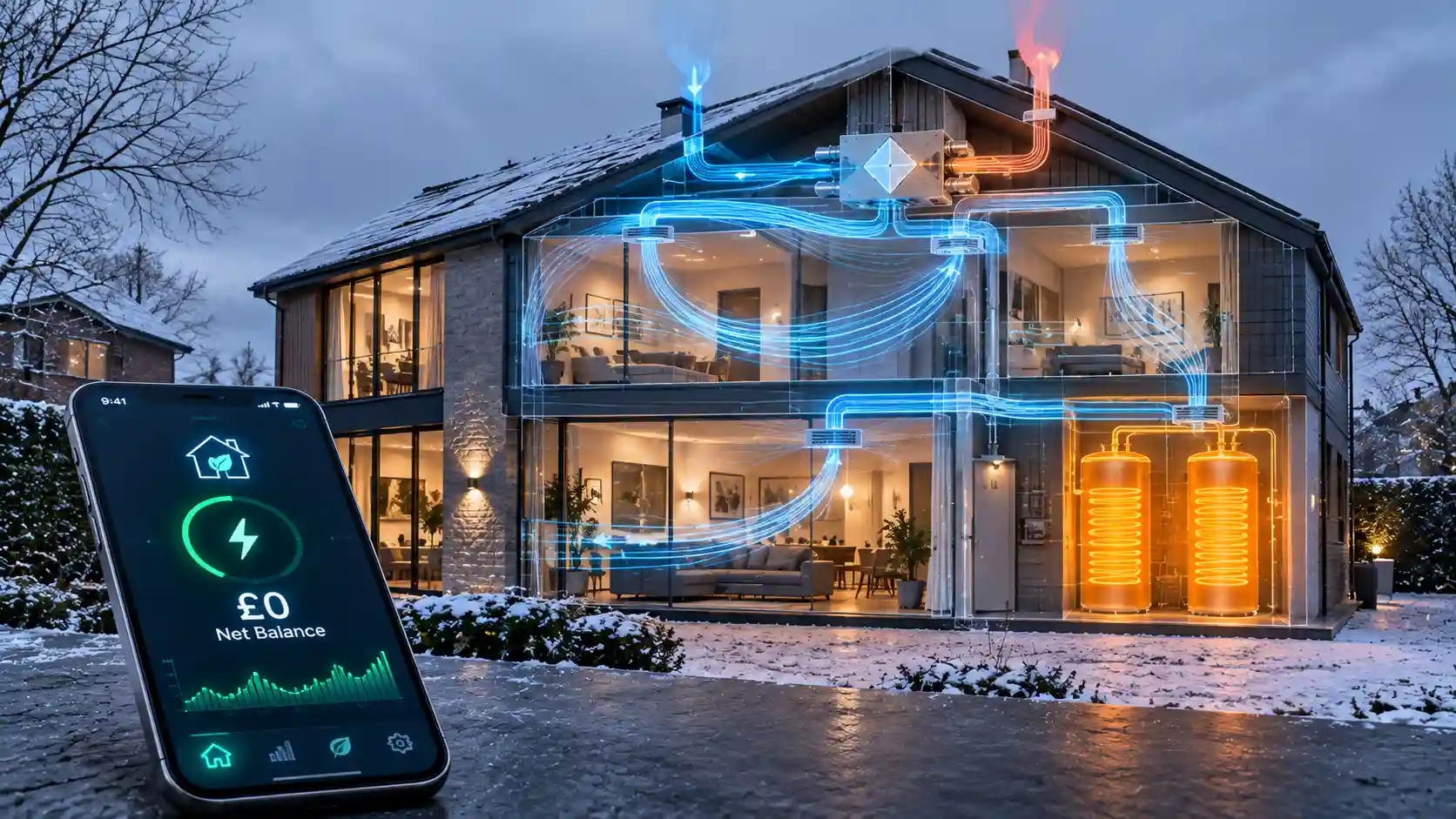
The proposition that a UK household can run its heating for free through the winter on rooftop solar alone does not survive contact with the astronomy. What can be engineered, however, is an annual net-zero energy balance in which a heavily upgraded building fabric, a low-temperature heat pump, controlled ventilation with heat recovery and a software-driven storage system convert the grid from a cost into a trading counterparty. This article audits that architecture for building services specifiers, micro-generation installers, residential decarbonisation consultants and energy asset managers. It works through the physics first, because every commercial claim in this sector is ultimately bounded by it. All numerical examples are standardised planning calculations for a representative four-bedroom detached house of about 150 m² treated floor area (TFA); they illustrate orders of magnitude and design logic rather than guaranteed outcomes for any specific property.
1. The Physics of the UK Winter Solar Deficit
Solar generation is governed by the geometry of the Earth’s axial tilt of 23.44 degrees. At a latitude of about 52.5 degrees north, typical of the English Midlands, the sun’s elevation at solar noon is given by 90 minus latitude plus declination. At the June solstice the declination is +23.44 degrees, giving a noon elevation of roughly 61 degrees. At the December solstice it is -23.44 degrees, giving about 14 degrees. At 56 degrees north, in central Scotland, the winter noon elevation falls to roughly 10.5 degrees.
Three compounding effects follow from that geometry. First, the beam irradiance incident on a horizontal surface scales with the sine of the elevation angle. The sine of 61 degrees is about 0.87, while the sine of 14 degrees is about 0.24, so the geometric flux per unit of horizontal area falls to roughly 28 per cent of the summer midday value before any atmosphere is considered. Second, the optical air mass, the path length of sunlight through the atmosphere relative to a vertical path, rises from about 1.15 at 61 degrees to about 4 at 14 degrees. Longer atmospheric paths increase Rayleigh scattering, aerosol absorption and water vapour absorption, so the direct-beam component is attenuated substantially more. Third, day length shrinks from about 16 hours 40 minutes in June to about 7 hours 50 minutes in December, so the integration window itself is less than half as long.
Multiplying these effects gives a clear-sky daily irradiation that is already in the region of 10 per cent of the summer figure on a horizontal plane. Tilting the array towards the low sun recovers part of that loss: a south-facing plane inclined at 35 to 40 degrees, a normal roof pitch, sees the winter sun at a much more favourable incidence angle than a flat plane, and a steep 60-degree tilt improves winter yield further at the cost of summer output.
Weather then compounds the deficit. In winter, a large majority of the available irradiance is diffuse rather than direct, because persistent stratiform cloud over the UK converts the beam component into scattered light. Diffuse irradiance is not concentrated at any particular angle, so the benefit of optimal tilt shrinks and the effective output is driven by the cloud optical depth and not by the geometry. Low sun angles also lengthen shadows, so neighbouring buildings, trees and roof features that are irrelevant in June can shade parts of an array for most of the day in December. Snow, frost and condensation add occasional further losses. A partial offset is that photovoltaic cells run more efficiently when cold, since the power temperature coefficient is around -0.3 to -0.4 per cent per kelvin, but this gains only a few per cent.
The practical outcome is expressed in specific yield. A well-sited, south-facing array in the south of England at a 35-degree tilt produces of the order of 900 to 1,000 kWh per kWp per year, with June delivering around 4 to 4.5 kWh per kWp per day and December around 0.5 to 0.7. For a 10 kWp array that implies approximately 40 to 45 kWh per day in June but only about 5 to 7 kWh per day in December and perhaps 6 to 9 kWh per day in January. That is a seasonal collapse of the order of 85 to 90 per cent between the extremes, and it is the reason why the generation profile is described as single-digit daily kWh across the core winter months. Many days in the depths of winter, under thick overcast, produce well below the monthly average, at one or two kWh in total.
The demand side is the mirror image. Space heating demand is concentrated in exactly the months in which solar yield is lowest, and within each day it peaks in the morning and evening when solar output is nil or negligible. A 10 kWp array that is generous in summer therefore delivers negligible instantaneous power to a heat pump working against a cold January evening. The system cannot be self-sufficient in winter. Instead, the design challenge is to make winter demand so small that its residual can be met cheaply from the grid at off-peak prices, while summer overproduction earns credit that offsets it over the year.
2. Building Fabric: U-Value Mathematics
The steady-state heat loss through a building element is Q = U × A × ΔT, where U is the thermal transmittance in W/m²K, A the area in square metres and ΔT the temperature difference in kelvin. U is the reciprocal of the total thermal resistance: U = 1 / (Rsi + R1 + R2 + … + Rse), where each layer’s resistance is its thickness divided by its thermal conductivity (lambda), and Rsi and Rse are the internal and external surface resistances, conventionally 0.13 and 0.04 m²K/W for walls.
Consider a typical 1970s detached house with an unfilled cavity brick and block wall. Its U-value is of the order of 1.0 W/m²K, equivalent to a total resistance near 1.0 m²K/W. Adding 200 mm of graphite-enhanced expanded polystyrene with a lambda of 0.032 W/mK contributes a resistance of 0.200 / 0.032 = 6.25 m²K/W. The new total resistance is about 7.25, so the U-value falls to approximately 0.14 W/m²K. The same target can be reached with about 140 mm of rigid PIR at lambda 0.022 (R = 6.4) or around 220 mm of wood-fibre board at lambda 0.040 (R = 5.5), where a vapour-open construction and embodied-carbon considerations are priorities. Solid brick walls with an initial U-value near 2.1 W/m²K require thicker layers, typically 220 to 250 mm of insulation, to reach the same figure.
The standards that govern deep retrofit are the Passivhaus Institute’s EnerPHit criteria. For a cool-temperate climate such as the UK, the component method specifies opaque elements with insulation of approximately 0.15 W/m²K or better where insulation is external, installed window U-values of 0.85 W/m²K or better, and a heat recovery efficiency of 75 per cent or better for the ventilation unit. The alternative is the whole-building route, which caps annual space heating demand at 25 kWh/m² of treated floor area. This is the performance target against which the rest of this article is calibrated. By comparison, a typical unimproved detached house has a space heating demand of 120 to 150 kWh/m² per year.
The element-by-element target specification for this house is as follows:
- External walls: 0.12 to 0.15 W/m²K, using 200 mm of external insulation with a mineral or silicone render, or a breathable wood-fibre system, with thermal bridging addressed at reveals, eaves, verges and foundation plinths.
- Loft and roof: 0.09 to 0.12 W/m²K, requiring roughly 400 to 450 mm of mineral wool at lambda 0.040 (R = 10 to 11), laid in crossed layers to avoid bridging by the ceiling joists.
- Ground floor: 0.12 to 0.15 W/m²K, achievable by lifting and replacing a solid floor with insulation of 120 to 150 mm, or by suspended-floor insulation and a draught-proofed void.
- Windows and doors: installed Uw of 0.8 to 0.85 W/m²K for triple glazing with warm-edge spacers and insulated frames, with a g-value of about 0.5 to preserve useful winter solar gain, and with the frame positioned within the insulation plane to avoid reveal bridging.
- Airtightness: 1.0 air changes per hour at 50 Pa for EnerPHit, or 0.6 for new-build Passivhaus, delivered with a continuous, tested air barrier and verified through blower-door testing.
A worked calculation illustrates the effect. Assume 140 m² of net external wall, 75 m² of roof, 75 m² of ground floor and 30 m² of glazing. In the unimproved condition, walls at 1.0, roof at 0.4, floor at 0.7 and windows at 2.8 W/m²K give a fabric loss of about 306 W/K. Adding ventilation at 0.7 air changes per hour of a 375 m³ volume, using the volumetric heat capacity of air of 0.33 Wh/m³K, contributes a further 87 W/K, for a total of roughly 393 W/K. With an annual heating degree-day total of about 2,200 kelvin-days, the gross annual demand is 393 × 24 × 2,200 / 1,000 = approximately 20,750 kWh, or around 138 kWh/m² after division by the 150 m² floor area.
After an EnerPHit-standard retrofit, the fabric components become 140 × 0.14 (19.6) for walls, 75 × 0.10 (7.5) for the roof, 75 × 0.15 (11.3) for the floor and 30 × 0.85 (25.5) for windows, a sum of 63.9 W/K. Allowing about 8 W/K for residual linear thermal bridges takes this to roughly 72 W/K. Ventilation losses, with 150 m³/h of controlled flow and 85 per cent effective heat recovery, are 0.33 × 150 × 0.15 = 7.4 W/K, plus approximately 6 W/K of residual infiltration. The total is close to 85 W/K, a reduction of almost 78 per cent. The gross annual demand is then 85 × 24 × 2,200 / 1,000 = about 4,490 kWh. Useful solar and internal gains of around 1,700 kWh bring the net space heating requirement to approximately 2,800 kWh, or about 19 kWh/m² per year, comfortably inside the 25 kWh/m² threshold.
Two engineering cautions apply. Moisture risk must be assessed for every retrofit build-up, particularly when adding impermeable insulation to the outside of a masonry wall with a damp-sensitive interior or internal insulation to solid walls, using hygrothermal simulation to verify that interstitial condensation does not occur. Thermal bridging is also disproportionately important: a linear transmittance of 0.3 W/mK at an unaddressed window reveal or wall-floor junction can easily add 10 to 20 W/K, enough to erase a fifth of the gains from the fabric upgrade.
3. Thermal Mass, Time Constants and the House as a Battery
A well-insulated envelope changes more than the heating load; it changes the dynamic behaviour of the building. The thermal time constant, tau = C / (UA), is the ratio of the effective thermal capacity of the structure to its heat loss coefficient. A heavy masonry house with an effective capacity of about 15 kWh/K and a loss of 393 W/K has a time constant of roughly 38 hours. The same house after retrofit, with a loss of 85 W/K, has a time constant of around 175 hours, over a week. Internal temperatures then drift slowly, at around 0.1 K per hour in the absence of heating on a cold day, so the building can coast through an expensive peak tariff window without noticeable comfort loss.
This is the foundation of load shifting. Pre-heating the thermal mass during a cheap overnight window stores energy in the structure for use throughout the day, and the cost of this storage per kWh is much lower than that of a chemical battery. Controls must nonetheless be set to avoid over-heating, to respect comfort limits and to account for the lag of mass-heavy floors and walls.
4. MVHR Thermodynamics
Mechanical ventilation with heat recovery supplies fresh air continuously while recovering most of the heat from the extracted stale air. In a counterflow plate heat exchanger, the supply and extract airstreams flow in opposite directions through thin, alternating channels separated by a conductive membrane. The counterflow arrangement maintains a temperature difference along the whole length of the exchanger and so permits a theoretical effectiveness approaching 100 per cent in a long core, which is why a modern unit can reach 90 per cent or more.
Sensible heat recovery effectiveness is defined as eta = (T_supply - T_outdoor) / (T_extract - T_outdoor). With an extract temperature of 21 degrees and an outdoor temperature of 0 degrees, an effectiveness of 90 per cent produces a supply temperature of about 18.9 degrees, which is why the incoming air does not feel cold. The ventilation heat loss is H = 0.33 × V_dot × (1 - eta) × ΔT. For a flow of 150 m³/h, 0.33 × 150 × 21 gives 1,040 W without recovery but only about 104 W with 90 per cent recovery, a saving of nearly 940 W continuously through the coldest weather. Over a heating season this represents several thousand kWh of avoided heating demand compared with natural or extract-only ventilation of the same air change rate.
Several practical effects reduce the performance in real installations compared with laboratory figures. Duct heat losses and leakage between the supply and extract paths reduce the in-use effectiveness, and so do imbalance between supply and extract flows and the temperature of the air in poorly insulated duct runs through cold loft spaces. Real-world effective figures are typically 80 to 88 per cent, and certified Passivhaus units are tested to a standardised protocol that accounts for leakage and imbalance. Fan electrical consumption matters too, because it is a continuous parasitic load; the specific fan power should be at or below about 0.45 Wh/m³, and efficient EC motors on low-resistance duct designs typically achieve 0.25 to 0.40. At 150 m³/h and 0.35 Wh/m³, the fans draw about 52 W, or around 460 kWh per year, which must be considered in the annual energy balance but is far smaller than the heat recovered.
In cold weather, the extract air can condense on the cold surfaces of the heat exchanger and, where the exhaust-air temperature falls below 0 degrees, can freeze. Frost protection is therefore needed, typically by reducing the supply flow temporarily, by using a small electric pre-heater or by bypassing part of the flow. Condensate must be drained, and a summer bypass should prevent the unit from warming incoming air on warm days. Filters at both the supply and the extract need regular replacement, because a clogged filter increases pressure drop, raises fan power and degrades the balance between the airstreams. Ventilation rates should be commissioned to a standard such as 30 m³/h per person or the room-by-room requirements of the building regulations, and boosted in kitchens and bathrooms.
5. Air-Source Heat Pump Performance in Sub-Zero Conditions
The coefficient of performance of a heat pump is the ratio of heat delivered to electrical energy consumed. The theoretical Carnot limit for heating is COP = T_hot / (T_hot - T_cold), with temperatures in kelvin. For a flow temperature of 35 degrees (308 K) and an outdoor air temperature of 7 degrees (280 K), the Carnot limit is 308 / 28 = 11. At -5 degrees (268 K), it is 308 / 40 = 7.7. Real machines achieve a fraction of the Carnot figure, typically 40 to 50 per cent for current inverter-driven units, giving practical values of around 4.5 to 5 at 7 degrees outdoors and 35 degrees flow, and roughly 2.8 to 3.2 at -7 degrees outdoors and 35 degrees flow.
The sensitivity of COP to flow temperature is as significant as the sensitivity to ambient. Raising the flow temperature from 35 to 50 degrees at an outdoor temperature of 0 degrees reduces the Carnot limit from 8.8 to 6.5 and the practical COP from about 3.7 to about 2.8. Every degree of unnecessary flow temperature costs roughly 2 to 3 per cent in efficiency. A house with a space heating load of 19 kWh/m² and a peak heat loss at a design outdoor temperature of -3 degrees of around 2 kW can be heated with a flow temperature of 30 to 35 degrees through underfloor heating or oversized low-temperature radiators, which keeps the seasonal performance factor high, at 3.5 to 4.5 compared with 2.5 to 3 for a poorly insulated property that needs 50 degrees or more.
Several additional mechanisms degrade winter performance. Between approximately 0 and 5 degrees, with high relative humidity, frost forms on the outdoor coil, restricting airflow and reducing heat transfer. The heat pump then runs a defrost cycle, briefly reversing and drawing heat from the building to melt the ice. Defrost cycles reduce the average COP over the period by several per cent and can briefly depress the delivered output. Inverter compressors modulate their output to match demand, but each has a minimum modulation limit; an oversized unit installed in a very low-load house will short-cycle, wasting energy and reducing life. Correct sizing, using a room-by-room heat loss calculation to MCS or equivalent standards, is therefore essential, and a high-performance fabric calls for a small unit, often 3 to 5 kW. Weather compensation, which reduces the flow temperature as outdoor conditions warm, and a low-temperature hot water strategy, using a legionella cycle only when needed, protect seasonal efficiency further.
Domestic hot water adds a load of around 2,000 to 2,500 kWh per year for a four-person household, or 6 to 8 kWh per day. Heating a cylinder to 50 or 55 degrees demands a higher flow temperature than space heating and so lowers COP, at around 2.5 to 3 on average. Schedule it in the cheap overnight window, ideally combined with a thermal store that holds the heat for the day.
6. Comparative Matrix: Building Optimisation Variants in a January Baseline
The matrix compares four configurations of the same representative property. Thermal demand is derived from the steady-state calculations above for a mean January outdoor temperature of about 4.5 degrees, with useful gains deducted. Cost estimates are indicative, based on planning assumptions of approximately 25p/kWh for standard-rate electricity, 6.5p/kWh for off-peak electricity, 6p/kWh for gas, an export rate of about 15p/kWh and total standing charges of around £15 per month for electricity. They are not forecasts of any particular supplier’s tariff.
| Building Optimization Envelope Variant | Average Daily Winter Thermal Demand (kWh) | Active Ventilation Strategy | Electrical Infrastructure Architecture | Seasonal Grid Interaction Profile | Net Monthly Operating Cost Profile (January Baseline) |
|---|---|---|---|---|---|
| A. Unimproved 1970s baseline: unfilled cavity walls, 100 to 150 mm loft insulation, older double glazing, gas boiler | Approximately 140 kWh space heating plus 6 to 8 kWh hot water (about 393 W/K heat loss coefficient) | Natural infiltration, trickle vents and extract fans, with uncontrolled air change of 0.5 to 0.9 per hour and no heat recovery | Single-phase supply, gas boiler, no generation and no storage | Full import of gas and electricity at peak daytime rates, with no export and no flexibility | Approximately £400 to £450 including gas and electricity standing charges |
| B. Partial retrofit: cavity fill, 270 mm loft, new double glazing, air-source heat pump on a standard tariff | Approximately 85 to 90 kWh space heating plus hot water (about 260 W/K heat loss coefficient) | Trickle vents and intermittent extract, uncontrolled infiltration of about 0.5 air changes per hour | Heat pump with radiators at 45 to 50 degrees flow, no generation, no storage | Full electrical import at standard rates, no export, high winter peak demand | Approximately £300 to £360, with seasonal efficiency limited by high flow temperatures |
| C. EnerPHit-standard envelope: 0.14 W/m²K walls, 0.10 roof, triple glazing, MVHR, low-temperature heat pump, time-of-use tariff | Approximately 24 kWh space heating plus 6 to 8 kWh hot water (about 85 W/K heat loss coefficient) | Balanced MVHR with 85 to 90 per cent sensible heat recovery, summer bypass and frost protection | Heat pump at 30 to 35 degrees flow via underfloor heating, no on-site generation, smart controls | Import only, with substantial load shifting into off-peak windows using building thermal mass | Approximately £90 to £130 at a blended import rate of roughly 12 to 17p/kWh |
| D. EnerPHit envelope plus 10 kWp solar, 15 to 30 kWh stationary battery, thermal storage and automated arbitrage | Approximately 24 kWh space heating plus 6 to 8 kWh hot water, with the same fabric as variant C | Balanced MVHR with 85 to 90 per cent sensible heat recovery, boosted automatically against humidity and CO2 sensors | 10 kWp array, hybrid inverter, lithium iron phosphate or sodium-ion battery, phase-change or ceramic thermal store, heat pump, half-hourly smart metering | Winter: off-peak import with overnight battery and thermal store charging. Summer: large export surplus that builds annual credit | Approximately £25 to £45 in January, mostly standing charge, with annual net energy cost near zero or slightly negative after summer export credit |
Variant D does not remove the fixed standing charge, which in the planning assumptions is around £180 to £200 per year and is the irreducible floor of any grid-connected bill. A genuinely £0 annual bill therefore depends on export revenue exceeding the sum of import costs and standing charges, which is plausible for a well-designed system but depends on tariff structures that are outside the designer’s control.
7. Sizing the Electrical Architecture
For variant D, the January electrical demand can be assembled from the components above. Space heating of about 24 kWh thermal per day at an average January COP of 2.8 is 8.6 kWh of electricity. Hot water of 7 kWh at a COP of 2.7 is 2.6 kWh. Ventilation fans add about 1.3 kWh. Lighting, cooking, appliances and standby loads contribute around 6 to 8 kWh, giving a total of about 19 to 21 kWh per day, or roughly 590 to 650 kWh across the month. A 10 kWp array yielding 6 to 9 kWh per day in January supplies around 190 to 280 kWh, offsetting about a third of the total. Because much of that solar arrives at midday, when demand may be low, it is stored in the battery or the thermal store for use in the evening.
The residual grid import is therefore about 350 to 450 kWh in January. If the battery and thermal store are charged in the off-peak window, almost all of this is purchased at roughly 6.5 to 7p/kWh, a cost of £23 to £31, to which the standing charge of about £15 is added. The comparison with an uncontrolled alternative is stark: the same 600 kWh bought at 25p/kWh would cost about £150.
Annual figures show the other half of the equation. A 10 kWp array in the south of England produces around 9,000 to 9,500 kWh per year. Electrical demand for this house is in the region of 4,500 kWh, being roughly 1,000 kWh for space heating, 800 kWh for hot water, 460 kWh for ventilation and 2,300 kWh for other loads. If around 2,500 kWh of generation is consumed on site or through storage, the surplus of 6,500 to 7,000 kWh is exported, which at 15p/kWh produces about £975 to £1,050 of revenue. Annual imports of about 2,000 kWh at a blended rate of around 8p/kWh cost about £160, and standing charges are about £180 to £200. The net annual position is a small credit of several hundred pounds, which is the sense in which an annual net-zero bill is achievable. These results are sensitive to export tariffs, which have declined in recent years and are subject to change.
Inverter selection and electrical design deserve attention. A hybrid inverter with DC-coupled battery inputs avoids a conversion stage and typically improves round-trip efficiency by a few percentage points compared with an AC-coupled system, although AC-coupled retrofits remain common because they leave an existing array untouched. Ensure the inverter’s charge and discharge rating matches the battery, since an undersized inverter can throttle a cheap overnight charge window and prevent the store from filling. The main supply fuse and any export or import limits set by the distribution network operator must be checked, since a 100 A single-phase supply can be a constraint when a heat pump, battery charger and electric vehicle charger operate simultaneously.
8. Battery Storage and Degradation Kinetics Under Rapid Cycling
Arbitrage depends on cycling the battery daily, and the economics therefore depend on degradation. Lithium-ion cells age through two overlapping processes: calendar ageing, which proceeds with time and increases with temperature and with a high state of charge, and cycle ageing, which accumulates with throughput and depends on depth of discharge, charge and discharge rate and temperature. The principal mechanism is growth of the solid electrolyte interphase on the graphite anode, which consumes cyclable lithium and raises internal resistance. Its rate follows an Arrhenius-type temperature dependence, roughly doubling for every 10 degree rise in cell temperature, so a battery in an unheated loft in summer ages faster than one in a stable indoor environment.
Lithium iron phosphate chemistry is the dominant choice for stationary storage because of its tolerance of cycling: manufacturers commonly quote 6,000 or more cycles to 70 per cent of original capacity at 80 to 90 per cent depth of discharge under moderate rates and room temperature, and its thermal stability is superior to nickel-based chemistries. At one cycle per day, 6,000 cycles represents more than 16 years, so in practice calendar life and the warranty term, commonly 10 years, are the binding limits. Charging below 0 degrees can cause metallic lithium plating on the anode, which is irreversible and a safety concern, so batteries in unheated spaces must have heating or a charge-current derating at low temperature. Sodium-ion cells offer lower energy density but good low-temperature performance, no reliance on lithium, cobalt or nickel, and cycle lives that are approaching those of lithium iron phosphate, which makes them an increasingly credible option for fixed installations where volume is not constrained.
The cost of degradation can be expressed per kWh throughput. For an installed system of 15 kWh nominal and 14 kWh usable, costing about £5,000, with 6,000 cycles at 14 kWh each, the lifetime throughput is 84,000 kWh and the capital cost per kWh stored is about 6p. The round-trip efficiency of 90 per cent means that the energy bought at 6.5p/kWh effectively costs about 7.2p for each kWh delivered. A kWh discharged to avoid a 25p/kWh peak import therefore yields a gross margin of about 17.8p and a net margin after degradation of around 12p. A cycle of 14 kWh earns a net benefit of about £1.70 per day, or around £600 per year, before any additional value from export or grid services. The payback on the battery alone is therefore long, and the economic case is strongest when the battery is part of a system in which it also captures solar surplus and in which the fabric is already efficient.
Rapid cycling does not by itself damage a battery provided that the C-rate stays moderate. Overnight arbitrage charging at 0.25 to 0.5 C, meaning a full charge over two to four hours, is gentle by cell standards. The major avoidable stressors are high temperature, prolonged storage at 100 per cent state of charge and deep discharge to very low levels. A sensible management strategy holds the battery at 20 to 95 per cent in the normal band, tops out only when required for the next day’s forecast and avoids dwelling at full charge.
9. Thermal Storage: Phase-Change and Ceramic Systems
Thermal storage is far cheaper per kWh than electrochemical storage, and the heat pump can charge it at a good COP. A conventional hot water cylinder stores sensible heat at 4.18 kJ/kgK, or 1.16 kWh per cubic metre per kelvin; a 300 litre cylinder heated across a 25 kelvin span stores about 8.7 kWh. Phase-change materials store heat in the latent heat of melting at a nearly constant temperature, with paraffins and salt hydrates melting at 45 to 60 degrees and latent heats of roughly 180 to 250 kJ/kg, so a compact unit can store two to four times as much heat per litre as water across a narrow temperature window. Ceramic and brick-core storage heaters hold heat at several hundred degrees, but they deliver it by direct electric resistance and do not benefit from the heat pump’s COP, so they are better suited to rooms that are difficult to serve with water-based emitters.
Installed cost for thermal storage is commonly in the order of £15 to £60 per kWh, against about £300 to £400 per kWh for installed batteries, which makes it the lowest-cost way of moving heating demand into cheap periods. The constraint is that it only stores heat, so the value is limited to the heating and hot water share of the load, and standing losses of 1 to 2 kWh per day should be accounted for. In a variant D system, the heat pump runs in the off-peak overnight window, charges the thermal store and perhaps raises the fabric temperature by a degree, then switches to a low-output or idle state in the peak window while the store and the building’s own time constant carry the load.
10. Time-of-Use Tariffs and Algorithmic Control
Smart tariffs of the Intelligent Go type provide a low rate during a defined off-peak period, commonly for about six hours overnight, around 23:30 to 05:30, with additional low-rate periods available when smart charging is dispatched. Planning assumptions here use a 6.5p/kWh overnight rate and a standard daytime rate of about 25 to 28p/kWh, a spread of roughly 4:1. Actual rates change frequently, so a system should be designed to be profitable across a range of spreads and not tuned to one tariff.
Control software determines whether this spread is captured. Open-source tools such as Predbat, which runs within Home Assistant, optimise the battery plan by combining several inputs: half-hourly import and export rates, a solar generation forecast from a service such as Solcast, a load forecast derived from the household’s own history, the current state of charge and the battery’s efficiency and power limits. It then evaluates a large number of candidate charge and discharge schedules across a forecast horizon of 24 to 48 hours and selects the plan that minimises expected cost. Typical outputs include when to charge from the grid, when to hold charge in reserve, when to discharge to the house, and when to export.
The decision loop can be summarised as follows. At each 30-minute slot, the controller reads actual state of charge, the latest forecasts and the current tariff. It then simulates the remainder of the horizon under each candidate plan, tracking the energy balance for every slot: generation plus battery discharge plus grid import equals load plus battery charge plus export, with efficiency losses applied. The plan with the lowest cost metric wins and its first action is applied. Because forecasts are uncertain, a well-configured controller weights a pessimistic solar scenario, commonly a lower-percentile case, to avoid being left short in the evening, and holds an overnight margin of safety against forecast error. Where the thermal store and heat pump are exposed to the same optimiser through a controllable setpoint, the loop extends to heating by treating the thermal store as a second, cheaper battery with its own losses and limits.
Failure modes are worth specifying at design stage. Dependence on a cloud forecast and an internet connection means that the system must fail safe, falling back to a local schedule if communications drop. Tariff changes, for example a modified off-peak window, must be reflected in the configuration promptly. Large winter charge windows can trigger heavy import for a short period, so the network supply capacity and the inverter and charger limits must be checked. Reserve capacity should be retained for power cuts if backup is specified, which cuts into the arbitrage range.
11. Retrofit Costs, Sequencing and Risk
Deep retrofit costs vary widely with building form and condition, and any figures should be treated as ranges to be tested through a survey and quotations. Indicative UK costs for a detached house of this size are of the order of £25,000 to £45,000 for external wall insulation, £3,000 to £6,000 for loft work, £15,000 to £30,000 for triple glazing, £6,000 to £12,000 for an MVHR installation, £8,000 to £14,000 for an air-source heat pump system before grant support, £10,000 to £14,000 for a 10 kWp array, £4,000 to £8,000 for a battery, and £2,000 to £6,000 for thermal storage and controls. A whole-house EnerPHit-style retrofit can therefore reach £80,000 to £150,000, and it is typically financed through refinance of an existing mortgage, staged work or integration with planned maintenance.
Sequencing matters. Fabric should come first, because it determines the size of everything downstream: an oversized heat pump, battery and array are wasted capital in a well-insulated house. Airtightness work and ventilation must be designed together, since improving airtightness without adequate ventilation raises humidity and indoor air quality risk. Heat pump sizing should be based on the post-retrofit heat loss, and in a staged programme this may mean installing a smaller unit or specifying one capable of modulating down. Solar and battery can be added at any stage, but should be specified so that the system can expand.
The principal risks are performance gaps between design and as-built, moisture problems from poorly designed insulation build-ups, tariff changes that reduce the arbitrage spread or the export rate, and the technology risk of software that depends on third-party services. A quality-assurance regime using blower-door tests, thermographic surveys, commissioning records and metered monitoring against the design model helps close the performance gap. Monitoring is also what makes the asset manageable: half-hourly data on heat pump COP, battery cycles, import and export and indoor conditions allows the system to be tuned and its claims to be verified.
12. Conclusion
A free winter is not available from rooftop solar, because the astronomy forbids it: the sun is low, the days are short, the cloud is thick and the loads are highest exactly when generation is weakest. An annual net-zero bill is nevertheless within reach for the right property, and the route to it is an integrated system. A fabric reduced to roughly 85 W/K, with an EnerPHit-standard envelope, cuts the winter thermal demand by about 80 per cent. Balanced ventilation with 85 to 90 per cent heat recovery eliminates most of the ventilation loss. A low-temperature heat pump lifts the seasonal COP to 3.5 or more. Thermal and electrochemical storage, directed by an optimiser, shifts what remains into the cheapest half-hours of the day. The summer array, oversized relative to the home’s own needs, earns the credit that closes the annual balance.
For specifiers and installers, the lesson is one of order and integration: fabric, ventilation, heat pump, storage and control have to be designed as a single thermodynamic and financial system. For asset managers and consultants, it is that the value of a retrofit lies as much in the time profile of its demand as in the quantity. A house that uses little energy, uses it slowly and buys it when it is cheap is a very different asset from one that merely generates it.