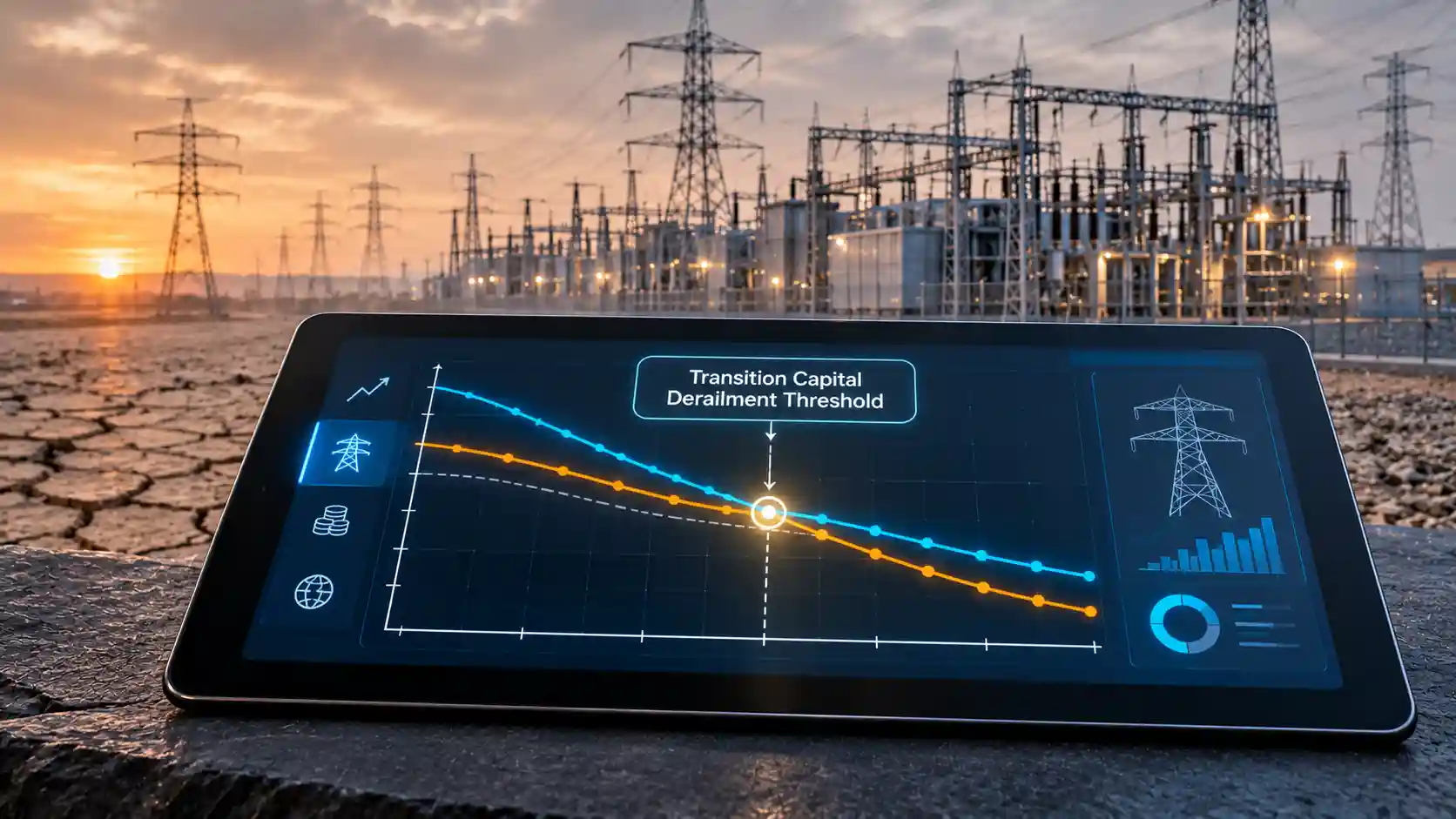
The conventional framing of climate risk separates it into transition risk (the cost of moving to a low-carbon economy) and physical risk (the cost of the climate changes that have already been locked in). For infrastructure asset managers and sovereign analysts, the more consequential insight is that the two are coupled. Physical shocks degrade the civil and mechanical assets on which the energy system runs, raise the cost of insuring and financing those assets, and strain the public balance sheets that would otherwise fund decarbonisation. The capital required for the transition is therefore reduced precisely when the need for it rises. This article refers to that coupling as derailment risk: the probability and magnitude of a feedback loop in which physical degradation cannibalises transition capital, which in turn leaves systems more exposed to further degradation. The audit below characterises each stage of the loop, from conductor physics and soil mechanics through to insurance capacity and sovereign credit spreads.
The Warming Baseline: What the Observational Record Actually Shows
Precision matters when describing the temperature record. The Copernicus Climate Change Service (C3S) and the World Meteorological Organization (WMO) both reported that 2024 was the first calendar year in which the global mean surface temperature exceeded 1.5°C above the 1850–1900 pre-industrial baseline, with C3S estimating the anomaly at approximately 1.6°C. Subsequent years have remained among the warmest on record. A single-year exceedance is not, however, the same as a breach of the Paris Agreement threshold, which is defined by reference to long-term averaging over roughly two decades. On that basis, long-term warming is currently assessed at approximately 1.3 to 1.4°C and is advancing at roughly 0.2°C per decade, which implies that the multi-decadal 1.5°C mark is likely to be crossed around the end of this decade or early in the next.
For asset managers, this distinction supports a practical conclusion. Individual years at or above 1.5°C are now part of the operating environment. Infrastructure is not sized to the long-term mean but to the extremes, and the extremes have shifted much more than the mean. A shift of a fraction of a degree in the average translates into a disproportionate change in the frequency of tail events, because the probability of exceeding a high threshold is highly sensitive to a shift in the distribution. A one-in-fifty-year heat event under the pre-industrial climate may occur roughly once per decade or more frequently under present conditions, with the design standards of existing assets still based on historic return periods.
Thermal Physics of Transmission Conductors
High-voltage overhead lines are among the most climate-exposed assets in the electricity system, because their performance is a direct function of ambient temperature. Two mechanisms operate: resistive loss and mechanical sag.
Resistance and delivery efficiency. The electrical resistance of aluminium-based conductors rises approximately linearly with temperature, R(T) = R20 × [1 + α(T − 20)], with a temperature coefficient α of about 0.004 per degree Celsius for aluminium. A conductor operating at 50°C therefore has a resistance about 12 per cent higher than the same conductor at 20°C reference, and at 80°C the figure is roughly 24 per cent. Because resistive loss is I2R, loss at constant current rises in direct proportion to resistance. Moving the operating temperature of a heavily loaded line from 50°C to 80°C increases its resistance by about 11 per cent (1.24 divided by 1.12). For a transmission corridor with typical technical losses of 6 per cent of delivered energy, that corresponds to an additional 0.6 percentage points, so delivery efficiency falls from about 94.0 per cent to about 93.4 per cent. The percentage looks small, but it is applied to very large energy flows and it coincides with peak demand, when marginal generation is most expensive and most carbon-intensive.
Thermal rating and ampacity. A more consequential effect is the loss of capacity. A conductor’s steady-state rating is set by the heat balance specified in standards such as IEEE 738 and CIGRE TB 601, in which resistive heating plus solar gain equals convective plus radiative cooling. Because the permissible conductor temperature is capped (commonly 75 to 90°C for ACSR conductors, beyond which the aluminium strands anneal and lose strength), a higher ambient temperature narrows the available temperature rise. To a first approximation, ampacity scales with the square root of the permitted temperature rise. If ambient temperature increases from 20°C to 40°C with a 75°C conductor limit, the available rise falls from 55 K to 35 K, and ampacity falls by a factor of roughly 0.80, a 20 per cent reduction in static capacity, before the effect of calm, low-wind conditions that typically accompany heat waves and further reduce convective cooling. Lines designed against seasonal ratings that assumed 30°C summer ambient temperatures are therefore being asked to carry load with no margin.
Sag and clearance. Conductors elongate with temperature at a coefficient of roughly 19 to 23 × 10−6 per kelvin. For a level span of length L and sag S, the conductor length is approximately L + 8S2/(3L), so small changes in length yield large changes in sag. Consider a 300 m span with 6 m sag at 20°C: the conductor length is about 300.32 m. Raising the conductor by 50 K lengthens it by about 0.29 m, which pushes sag to roughly 8.2 m, an increase of about 2.2 m or 37 per cent. Real conductors behave somewhat differently because tension reduces as sag increases and the steel core in ACSR carries a larger share of the load, but the order of magnitude holds. The practical result is reduced ground and vegetation clearance, with consequent flashover risk. Sag-related contact with trees and structures is a recognised contributor to major blackout events, and it forces system operators to constrain flows pre-emptively. Dynamic line rating, reconductoring with high-temperature low-sag (HTLS) conductors and structural uprating of towers are the principal mitigations, each with a capital cost that has to be funded from the same constrained budgets discussed later.
Geotechnical Mechanics: Soil Moisture Cycling and Foundation Fatigue
The second mechanical pathway operates below the surface. Many clay soils across the UK and continental Europe are shrink-swell soils: as moisture content falls, matric suction rises and the soil volume contracts; when rain returns, suction dissipates and the soil swells. High-plasticity clays such as London Clay and Gault can undergo volumetric change of 10 per cent or more across a moisture cycle, with associated vertical movements of tens of millimetres at the surface and ongoing movement at depths of several metres, particularly where vegetation roots extract moisture from the deep profile.
Climate change intensifies this cycle by increasing both its amplitude and its frequency. Prolonged drought dries the profile to depth and opens desiccation cracks, which in turn become preferential flow paths when intense rainfall arrives. The infiltration of water into a cracked, desiccated clay mass reduces its effective stress and shear strength rapidly, while the sudden positive pore pressures can trigger slope instability. The mechanics are those of progressive failure: each cycle weakens the soil structure slightly, reducing peak strength towards a lower residual strength, so that an embankment that survived a century of historic cycling may fail in a cycle of the same magnitude after a sequence of extreme wet and dry years.
Rail networks. Much of the UK rail network sits on Victorian earthworks that were built without modern compaction control, of variable fill quality and with limited drainage. Cuttings and embankments in high-plasticity clay are especially vulnerable to the wet-dry cycle. Seasonal shrink-swell movement degrades track geometry, producing vertical and lateral misalignment, requiring more frequent tamping and imposing temporary speed restrictions. Heat adds a separate failure mode: rails expand thermally and, if the rail temperature exceeds the stress-free neutral temperature by too great a margin (often 30 to 35 K or more), compressive stress can cause the track to buckle in a sun kink. The consequence is not only maintenance expenditure but also performance loss, which has an economic impact through delay and cancellation costs.
Transmission pylon footings. Lattice tower foundations, typically pad-and-chimney or pile designs, are sized for compressive, uplift and overturning loads under wind and ice. They are less tolerant of differential settlement. Seasonal soil shrinkage beneath one leg of a tower and not another introduces unplanned bending in the lattice members and redistributes leg loads, while saturation of the soil reduces uplift resistance, since the shear strength of the soil cone mobilised against uplift falls with increased moisture content. Erosion and scour around footings in river floodplains, where high flows undercut foundations, create a further category of failure. Repeated differential movements lead to fatigue in bolted connections and members, and require more frequent inspection, regrouting and underpinning.
Hydrological Constraints on Thermal and Nuclear Cooling
Thermal power stations are, in thermodynamic terms, heat engines that need a cold sink. In a Rankine cycle, the condenser temperature determines the back-pressure on the turbine, and each degree of increase in cooling-water temperature raises that back-pressure and reduces the available enthalpy drop across the turbine. As a rule of thumb, the net output of a once-through-cooled steam plant falls by in the order of 0.3 to 0.5 per cent for each degree Celsius of rise in condenser cooling-water temperature, with a larger effect where cooling towers have less approach margin in hot, humid conditions. The effect on efficiency is modest in the range of normal variation, but becomes material at the extremes.
The binding constraint, however, is regulatory. Plants located on inland rivers are subject to environmental discharge limits that cap the temperature of the receiving water downstream, to protect aquatic ecosystems whose oxygen solubility declines as temperature rises, and an upper limit on the temperature delta between the intake and the outfall. When river flows drop in drought, there is less water to dilute the plant’s warm effluent, and when the background river temperature rises, the headroom to the regulatory limit shrinks. Operators must then reduce output to remain compliant. French nuclear fleet operators have repeatedly curtailed output or applied for temporary derogations during recent summer heat waves, and similar constraints have affected plants on the Rhine, the Danube and in the American Southeast. During such events, curtailments of several gigawatts coincide with peak cooling demand and with reduced hydropower output, as well as with reduced wind output in blocking high-pressure conditions.
The economic consequences are several. Baseload capacity that was assumed to be firm becomes seasonally derated, which reduces the capacity credit that these plants hold in capacity markets. Replacement energy must be purchased at spot prices, which in scarcity conditions can be several multiples of the average. Low-carbon baseload is replaced with gas-fired generation, which raises emissions during the year, and increases exposure to fuel-price volatility. For investors, the point is that cooling-water availability is a stranded-asset variable that has seldom been priced into long-term valuations of thermal and nuclear assets. Adaptation options (cooling towers, hybrid wet-dry systems, relocation of intakes to cooler depths, and upstream storage) are all available, but their cost is high and they must be financed.
Comparative Matrix: Vulnerability, Forcing and Capital Impact
| Infrastructure Asset Vulnerability Vector | Physical Climate Forcing Mechanism | Accelerated Asset Depreciation Rate (Projected Delta) | Macro-Financial Risk Consequence | Impact Velocity on Transition Capital Allocation |
|---|---|---|---|---|
| Overhead transmission conductors and fittings | Elevated ambient and conductor temperature: higher resistance, sag, annealing and reduced ampacity (up to about 20% static capacity loss on a 20 K ambient rise) | Approximately +5% to +15% on annual charge where thermal cycling shortens conductor and fitting life | Higher technical losses, congestion costs and reconductoring capital expenditure; reliability penalties under regulated revenue regimes | Moderate to fast: rating losses appear immediately, while uprating programmes divert grid-reinforcement budgets within one to three years |
| Pylon footings and tower foundations | Wet-dry cycling of shrink-swell clays, scour and reduced uplift resistance under saturation | Approximately +10% to +25% in exposed clay and floodplain corridors, reflecting shortened foundation service life | Unplanned underpinning and failure repair costs; higher inspection regimes; outage-related penalties | Slow to moderate: damage is cumulative and often appears as step failures after extreme sequences |
| Rail embankments, cuttings and track | Pore-pressure cycling, desiccation cracking, progressive strength loss and thermal track buckling | Approximately +15% to +30% on earthworks in high-plasticity clay; faster renewal cycles for track components | Higher maintenance and renewal expenditure, speed restrictions, delay and compensation costs, freight disruption | Moderate: recurrent seasonal losses draw down renewals funding that competes with electrification budgets |
| Thermal and nuclear plant cooling systems | Lower river flow and warmer intake water, lowering condenser performance and breaching discharge limits | Approximately +5% to +10% effective reduction in utilisation and revenue-generating life, with additional adaptation capital | Loss of firm capacity, scarcity pricing, replacement fuel cost, capacity-market derating | Fast: curtailments occur within days of a drought-heat event, with re-pricing of capacity risk within one to two years |
| Insured property and public-asset portfolios (including sovereign balance sheets) | Clustered flood, subsidence, storm and heat losses that raise loss ratios and reinsurance costs | Approximately +10% to +20% effective increase in annualised asset consumption where uninsured or self-insured | Premium escalation, coverage withdrawal, protection gap, sovereign contingent liabilities and credit-rating pressure | Fast to very fast: reinsurance repricing is annual, and ratings and spread responses can follow a major event within months |
Matrix notes: the depreciation deltas are illustrative planning assumptions chosen to demonstrate order-of-magnitude exposure, and must be replaced by asset-specific condition data in any real valuation. They represent the increase in the annual depreciation charge that results from a shorter expected useful life.
Asset Depreciation Accounting Under Physical Climate Stress
For an asset with cost C, residual value R and expected useful life N years, the straight-line annual charge is (C − R)/N. If physical climate stress reduces the expected useful life by a fraction f, the new annual charge becomes (C − R)/[N(1 − f)], an increase of f/(1 − f). A 50-year asset whose expected life is revised down to 40 years (f = 0.20) therefore sees its annual depreciation charge rise by 25 per cent, and a revision to 35 years (f = 0.30) raises it by about 43 per cent. The sensitivity is non-linear because shortening life concentrates the cost recovery into a smaller denominator.
Beyond straight-line, there are more sophisticated approaches. Condition-based and units-of-use models adjust depreciation to measured degradation. Probabilistic approaches treat the asset’s remaining life as a distribution, with a hazard rate h(t) that is a function of cumulative environmental loading, such as the number of thermal exceedance hours or the number of wet-dry cycles. The expected loss is the integral of the hazard rate multiplied by the replacement cost, discounted at the appropriate rate. IAS 36 requires an entity to test for impairment when indicators arise, and IFRS S2 introduces disclosures regarding physical climate risk, so the effects described above have direct implications for reported asset values. For regulated utilities, the regulatory asset base is depreciated on agreed schedules, and a divergence between the economic life and the regulatory life is an exposure borne by the equity holder until the regulator recognises it.
Insurance Capacity and the Protection Gap
Insurance transmits physical losses into the financial system. Property and casualty insurers price on historical loss experience supplemented by catastrophe models, and reinsurers re-price annually. When secondary perils (floods, convective storms, wildfire, subsidence) produce persistent losses above model expectation, insurers respond through higher premiums, higher deductibles, narrower coverage and, in the extreme, withdrawal from high-risk postcodes or regions. Reinsurers have increased attachment points, reducing their exposure to frequency losses and returning them to the primary market.
The result is a widening protection gap: the share of economic losses that is uninsured. Globally, a majority of weather-related economic losses fall outside insurance cover, and the share is substantially higher in emerging markets. Where losses are uninsured, the residual falls on households, firms and governments. For infrastructure owners, the effect arrives through three channels: higher premiums, which reduce free cash flow; higher deductibles and exclusions, which increase retained risk; and, in the worst case, uninsurability, which can raise financing costs because lenders often make insurance a condition of their facilities. Project finance for renewable assets in flood-exposed or wildfire-exposed locations is increasingly dependent on an insurance market that is itself in retrenchment.
Sovereign Credit Risk and the Capital Cannibalisation Loop
Public balance sheets are the shock absorber of last resort. After a major event, governments fund emergency response, repair public infrastructure, and often provide relief to uninsured households and firms. These outlays are unbudgeted and frequently large relative to annual capital expenditure. In a simple fiscal identity, the capital available for proactive investment equals revenue, less recurrent expenditure, less debt service, less emergency and reconstruction spending. If the final term rises while revenues are flat or are themselves reduced by damage to the tax base, investment capacity falls.
A stylised illustration makes the mechanism concrete. Suppose a regional authority has a capital budget of 100 million pounds, of which 10 per cent is normally absorbed by reactive repairs, leaving 90 million for planned investment, of which, say, a third (30 million) is allocated to decarbonisation projects such as network upgrades, building retrofit and charging infrastructure. If a sequence of floods and heat events raises the reactive share to 25 per cent, planned investment falls to 75 million, and if decarbonisation retains its one-third share it falls to 25 million, a 17 per cent reduction. In practice, decarbonisation tends to be the more discretionary element, and so loses more than proportionally: if the full 15-point swing is taken from discretionary programmes, the decarbonisation allocation falls to 15 million, a 50 per cent cut. The effect compounds because deferred maintenance on resilience raises the probability and cost of the next event.
The credit channel reinforces this. Rating agencies, including Moody’s, S&P Global and Fitch, now incorporate physical climate exposure into sovereign and sub-sovereign assessments, and academic work has linked climate vulnerability to higher borrowing costs for exposed countries. A downgrade raises the yield demanded on new issuance, which raises debt service, which further reduces capacity for investment: a reinforcing loop. For a sovereign with debt of 100 per cent of GDP, a 50 basis point increase in average borrowing cost, when fully passed through, adds half a percentage point of GDP to annual interest costs, an amount comparable with the entire incremental public spending needed for a significant decarbonisation programme in many economies. Green bond issuers are exposed in two ways: the credit quality of the sponsor deteriorates, and the pipeline of eligible projects may stall as capital is redirected.
Modelling the Derailment Loop
The feedback structure can be summarised as a discrete-time system. Let Dt denote the cumulative physical damage stock, Kt the capital available for transition investment, and It the realised resilience-and-decarbonisation investment. Annual physical loss Lt is a function of hazard intensity and of the vulnerability of the asset base, which declines with the resilience investment: Lt = Ht × V(Dt, It-1). Public and private reconstruction spending Rt is a share of Lt net of insured recoveries. Available capital then follows Kt+1 = Kt − Rt − ΔDSt, where ΔDSt is the increase in debt service induced by spread widening. The loop is stable when investment reduces vulnerability enough that losses decline, and unstable when reconstruction and debt-service costs consume investment capacity faster than resilience can reduce losses. The threshold between the two regimes, the derailment point, depends on the ratio of annual loss to investable capital, the insured share and the sensitivity of spreads to loss.
Practitioners can approximate this with scenario analysis using the Network for Greening the Financial System (NGFS) scenarios and with asset-level hazard overlays, combined with credit transition matrices. The key output is not a point forecast but the identification of nonlinearities: asset classes and jurisdictions where a modest increase in hazard produces a disproportionate increase in loss, financing cost or both.
Implications for Asset Managers, Sovereign Analysts, Issuers and Investors
- Asset managers: replace historic design-basis assumptions with forward-looking hazard data; revise useful lives and depreciation schedules where evidence supports it; prioritise reconductoring, drainage and earthworks stabilisation where criticality is highest.
- Sovereign debt analysts: integrate physical loss ratios, insurance penetration and fiscal buffers into credit assessments; monitor the reactive share of capital expenditure as a leading indicator of crowding out.
- Green bond issuers: embed resilience criteria in eligible-project definitions, and disclose physical risk assessments under IFRS S2 or TCFD-aligned frameworks to protect investor confidence.
- Clean-energy venture capitalists: favour technologies that enhance system resilience (dynamic line rating, grid-forming storage, distributed generation, advanced conductor materials, moisture-resilient foundations and predictive maintenance), as they address the bottleneck directly.
Conclusion
The central finding of the derailment-risk framework is that physical climate impacts and transition finance cannot be analysed in separate silos. Conductor heating, soil-moisture cycling and cooling-water constraints are engineering phenomena with calculable effects on capacity, loss and asset life. Those effects are translated by accounting conventions, insurance markets and sovereign credit into constraints on the volume and cost of capital. The mechanics are neither speculative nor remote, and the governing relationships are well understood. What is uncertain is the speed and the location of the tipping points, which is precisely why the quantification of vulnerability, at the level of individual assets and jurisdictions, is the highest-value activity available to those allocating capital today.