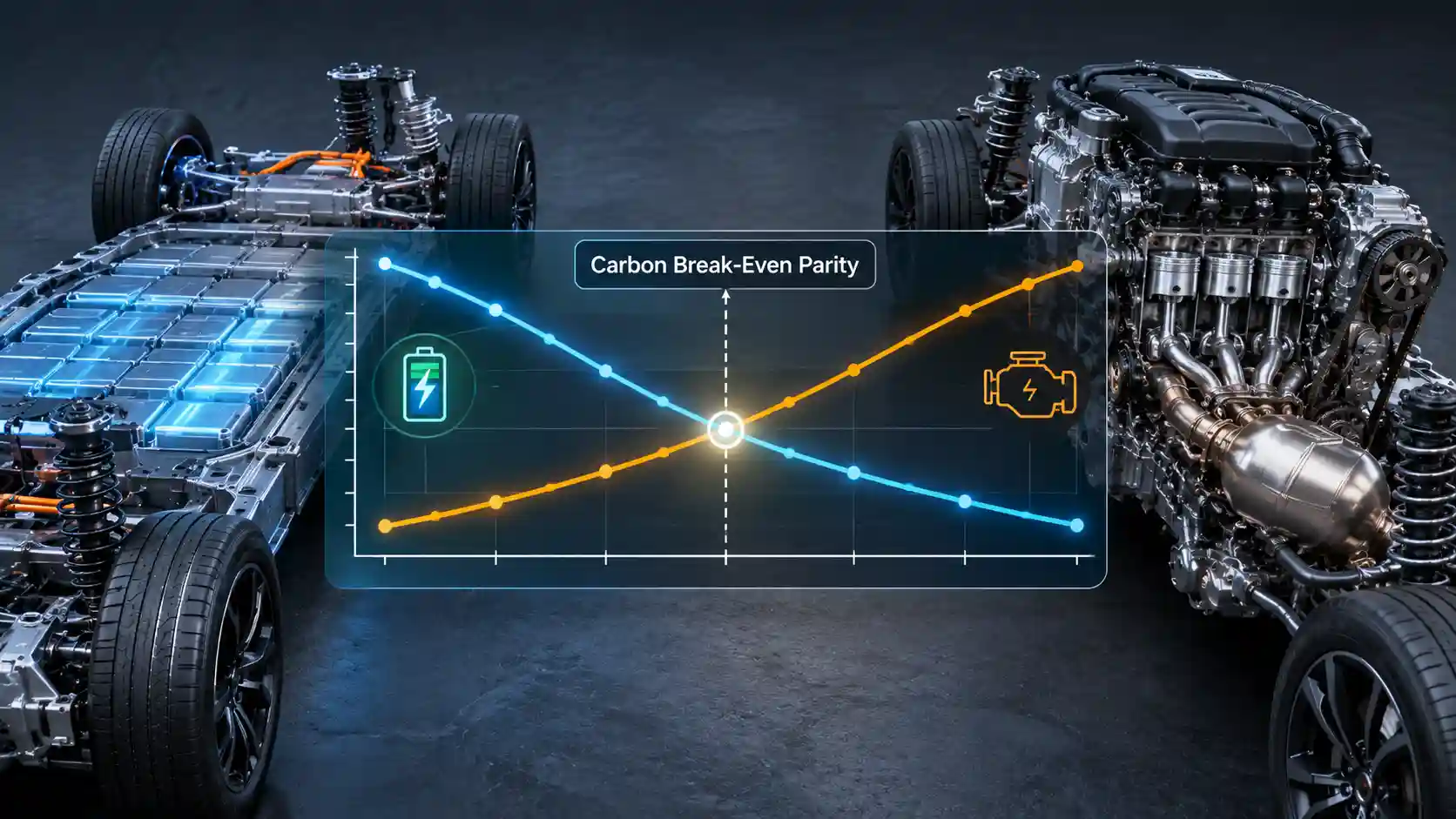
Tailpipe emissions are a convenient but incomplete metric. A defensible climate assessment of a battery electric vehicle (BEV) requires a full lifecycle accounting boundary: raw material extraction, refining, precursor synthesis, cell and pack manufacture, vehicle assembly, operational energy supply, maintenance and end-of-life treatment. This audit decomposes the manufacturing debt that a 2026 BEV carries when it leaves the factory, models how the carbon intensity of the charging supply determines the speed at which that debt is repaid, and quantifies the whole-life advantage over a comparable petrol vehicle. All figures are expressed in carbon dioxide equivalent (CO2e) using 100-year global warming potentials, and are consistent in order of magnitude with published International Energy Agency (IEA) and International Council on Clean Transportation (ICCT) lifecycle work.
Defining the Accounting Boundary and the Real Meaning of Carbon Debt
The term “carbon debt” is used in two distinct ways, and conflating them is the most common source of error in public debate. The first is the gross battery debt: the emissions attributable to producing the traction battery itself. For a 75 kWh pack, with cell production specific emissions in the region of 90 to 120 kg CO2e per kWh of capacity depending on chemistry and the carbon intensity of the supply chain, this amounts to roughly 7 to 9 tonnes of CO2e. This is the figure that appears in headlines.
The second is the net manufacturing penalty: the difference between the total production footprint of the BEV and that of a comparable internal combustion engine (ICE) vehicle. A BEV does not require an engine block, multi-speed gearbox, exhaust system, catalytic converter, fuel tank or the associated casting, machining and precious-metal catalysis. These omissions offset a substantial part of the battery debt. After netting them off, a typical mid-sized BEV leaves the factory with a total production footprint of approximately 11 to 13 tonnes CO2e, against roughly 8 to 9 tonnes for the ICE equivalent: a total manufacturing footprint around 30 to 40 per cent higher, and a net excess of approximately 2.5 to 3.5 tonnes. Parity calculations must use the net excess, because that is the quantity the operational savings actually have to repay.
Thermodynamics of Cathode Production: NMC and LFP Compared
The cathode is the single most carbon-intensive component of the cell, typically accounting for 35 to 45 per cent of cell-level emissions. Its footprint is governed by the energy needed to drive endothermic reactions at high temperature, and by the carbon intensity of the electricity and process heat that supplies that energy.
Nickel-rich NMC (for example NMC811). Nickel is extracted either from sulphide ores, concentrated and smelted pyrometallurgically, or from laterite ores by high-pressure acid leaching (HPAL) or rotary kiln-electric furnace routes. Laterite processing in regions served by coal-fired captive power is the most emissions-intensive pathway, and can exceed 20 tonnes CO2e per tonne of contained nickel. Smelting furnaces operate above 1,400°C. Cobalt, usually a by-product of copper or nickel mining, adds both smelting energy and the fugitive emissions associated with sulphide roasting. Manganese sulphate production requires sulphuric acid leaching and crystallisation, with significant steam demand.
Lithium arrives as hydroxide for nickel-rich chemistries. Hard-rock spodumene must be calcined at around 1,050°C to convert the alpha phase to the leachable beta phase, then acid-roasted at roughly 250°C and leached, before conversion and crystallisation. Brine routes avoid the calcination step but consume large quantities of reagents and evaporation or direct-extraction energy. The three metals are then co-precipitated as a mixed hydroxide precursor (pCAM) in stirred reactors under tightly controlled pH, temperature and ammonia chemistry; the ammonia, sodium hydroxide and heated wash water all carry upstream emissions. Finally, the precursor is blended with lithium hydroxide and calcined in an oxygen-rich atmosphere at 700 to 900°C for ten hours or more. Nickel-rich layered oxides require the oxygen atmosphere to suppress cation mixing, and the long dwell times in roller-hearth kilns make this step highly electricity- and gas-intensive.
Iron-rich LFP. Lithium iron phosphate avoids nickel and cobalt entirely. Its precursor chain involves iron phosphate synthesis from iron sulphate or iron metal and phosphoric acid (itself derived from wet-process or thermal phosphate rock processing), followed by mixing with lithium carbonate and a carbon source, then carbothermal sintering at approximately 650 to 800°C under an inert nitrogen atmosphere. The absence of nickel smelting and cobalt refining means that LFP cathode active material typically carries a materially lower footprint per kWh. This is partly offset by the lower gravimetric energy density of LFP cells, which requires more cell mass per kWh, but pack-level analyses generally still favour LFP by 15 to 30 per cent on a per-kWh basis, with the advantage widening where nickel is sourced from coal-powered laterite plants.
Anode and other components. Synthetic graphite is produced by graphitising petroleum coke or needle coke at 2,800 to 3,000°C in Acheson or lengthwise-graphitisation furnaces for days at a time. It is among the most energy-intensive steps in the entire cell chain, and the origin of the electricity matters enormously. Aluminium for housings and the pack enclosure, copper foil for the anode current collector, and electrolyte salts such as LiPF6 each contribute additional embedded emissions. Aluminium smelted with hydropower carries a fraction of the footprint of coal-powered production, a distinction that explains why identical battery designs can differ by a factor of two in measured carbon intensity.
Cell Manufacture: Clean-Room and Dry-Room Energy Demand
Cell assembly is dominated not by chemistry but by environmental control. Lithium-ion electrodes are coated as slurries, and in nickel-rich systems N-methyl-2-pyrrolidone (NMP) is the usual cathode solvent. Coated electrodes pass through long drying ovens, and the evaporated NMP must be captured and recovered by condensation or adsorption. Electrolyte filling, however, requires an atmosphere with a dew point of minus 40°C to minus 60°C, equivalent to a relative humidity well below one per cent, because LiPF6 hydrolyses on contact with moisture to form hydrofluoric acid and degrades cell performance. Maintaining those dry rooms means continuous desiccant-wheel regeneration with heated air, together with chilled-water cooling and HEPA filtration to control particulates that could cause internal short circuits.
Formation and ageing add further load. Each cell must be charged and discharged under controlled conditions for days to form the solid-electrolyte interphase, an electricity consumption that is partly recoverable but often is not. Aggregate gigafactory energy demand is commonly cited in the range of 40 to 60 kWh of electricity-equivalent per kWh of cell capacity, with thermal demand for drying and dehumidification being a major component. Where that energy is supplied by a coal-heavy grid, such as those serving large parts of East Asian cell production, cell-stage emissions can be double those of a plant powered by hydro, nuclear or wind. This is why siting and power purchasing strategy are now first-order carbon accounting variables for manufacturers, and why European and North American gigafactories report materially lower specific emissions than the global average.
Greenhouse gases arising across this chain are not limited to CO2. Methane is released through coal mining and gas supply that feed process heat and power; nitrous oxide arises from nitric-acid-based reagent chains and certain combustion processes; and fluorinated gases may be released during semiconductor-like manufacturing steps for power electronics. All are weighted into the CO2e total, though CO2 from fuel combustion and electricity generation remains the dominant component.
Vehicle Assembly and Whole-Life Tracking
Beyond the pack, a BEV body-in-white uses steel and aluminium in quantities comparable with an ICE vehicle, with growing use of large single-piece castings that cut part counts and joining energy. Paint shops, which require heated ovens and conditioned air, represent a significant share of assembly energy regardless of powertrain. Permanent-magnet synchronous motors introduce rare-earth supply chains (neodymium, dysprosium), while power electronics add silicon or silicon-carbide semiconductor wafers whose fabrication is electricity-intensive. For carbon accounting directors, the practical implication is that the vehicle should be tracked through a bill-of-materials approach with supplier-specific emission factors, not generic averages. Product-level reporting under the EU Battery Regulation’s carbon footprint declaration requirements is moving the market in precisely this direction.
End-of-life treatment also matters. Recovery of nickel, cobalt, copper and lithium by hydrometallurgical or pyrometallurgical recycling displaces primary production at a fraction of the energy cost, and credits of 10 to 30 per cent against the battery manufacturing footprint are plausible as recycled content rises. These credits are excluded from the headline parity figures in this article, so the results are conservative.
Operational Emissions: The Mathematics of Payback
Payback is a straightforward ratio. Let the net manufacturing excess be M (kg CO2e), the ICE emissions per mile be Eice, and the BEV emissions per mile be Eev = c × g, where c is the electricity consumed per mile from the wall (including charging losses) and g is the grid carbon intensity in kg CO2e per kWh. The break-even distance is then D = M / (Eice − Eev).
For the comparator, a petrol car achieving 40 mpg burns roughly 0.114 litres per mile. With about 2.3 kg of CO2 per litre at the tailpipe and an upstream (well-to-tank) uplift of around 20 per cent for extraction, refining and distribution, Eice is approximately 0.31 kg CO2e per mile. For the BEV, a mid-sized 2026 model consuming 0.30 kWh per mile at the wall gives Eev = 0.30 × g. At a UK grid intensity of about 150 g/kWh (0.15 kg/kWh) Eev is only 0.045 kg per mile, a saving of roughly 0.265 kg per mile. Divide a net excess of 2.5 to 3.5 tonnes by that saving and the parity distance is approximately 9,400 to 13,200 miles. For a driver covering 12,000 miles a year, break-even arrives in about 9 to 13 months; for a lower-mileage driver covering 7,000 miles a year it extends to around 16 to 23 months. This is the origin of the commonly cited range of one to two years of typical driving.
Comparative Matrix: Grid Topology and Payback Trajectories
| Charging Grid Infrastructure Topology | Average Carbon Intensity (g CO2e/kWh) | Upfront Battery Manufacturing Debt (75 kWh Basis) | Kilometre/Mile Parity Break-Even Horizon | Lifetime GHG Reduction vs. Petrol Asset (15-Year Basis) |
|---|---|---|---|---|
| Hydro-dominant grid (Norway, Quebec, Iceland) | Approximately 20–30 | Approximately 7–9 t CO2e gross (net excess approx. 2.5–3.5 t) | Approx. 8,300–11,600 miles (13,400–18,700 km); 7–12 months at 12,000 miles a year | Approximately 73% |
| Domestic rooftop solar PV (behind-the-meter, direct charging) | Approximately 40–50 (lifecycle panel emissions only) | Approximately 7–9 t CO2e gross (net excess approx. 2.5–3.5 t) | Approx. 8,400–11,800 miles (13,500–19,000 km); 7–12 months at 12,000 miles a year | Approximately 72% |
| UK national grid (falling towards ~150) | Approximately 150 | Approximately 7–9 t CO2e gross (net excess approx. 2.5–3.5 t) | Approx. 9,400–13,200 miles (15,100–21,200 km); 9–13 months at 12,000 miles a year | Approximately 63% |
| European Union average mix | Approximately 230 | Approximately 7–9 t CO2e gross (net excess approx. 2.5–3.5 t) | Approx. 10,400–14,500 miles (16,700–23,300 km); 10–14 months at 12,000 miles a year | Approximately 57% |
| United States average mix | Approximately 370 | Approximately 7–9 t CO2e gross (net excess approx. 2.5–3.5 t) | Approx. 12,600–17,600 miles (20,300–28,300 km); 13–18 months at 12,000 miles a year | Approximately 46% |
| High-coal grid (coal-dominant systems) | Approximately 700 | Approximately 7–9 t CO2e gross (net excess approx. 2.5–3.5 t) | Approx. 25,000–35,000 miles (40,000–56,000 km); 25–35 months at 12,000 miles a year | Approximately 21% |
Matrix notes: the break-even range reflects the 2.5 to 3.5 tonne net excess; lifetime reductions assume a net excess of 3 tonnes, an ICE manufacturing footprint of 8.5 tonnes, 0.31 kg CO2e per mile for the petrol vehicle, 0.30 kWh per mile for the BEV and a static grid intensity over the 15 years. All figures are illustrative modelling outputs and will vary with vehicle specification, driving pattern and the decarbonisation trajectory of each grid.
Grid Intensity as the Dominant Operational Variable
The matrix shows that the payback slope is controlled almost entirely by the grid term. At 150 g/kWh, each mile driven repays 0.265 kg of the debt; at 700 g/kWh, only 0.10 kg. The relationship is linear in g, but because the denominator in D is the difference between ICE and BEV emissions, it becomes strongly non-linear as BEV emissions approach those of the ICE comparator. The break-even distance would be infinite at a grid intensity of around 1,030 g/kWh with these assumptions, which marks the theoretical ceiling at which a BEV would offer no benefit at all. No national grid operates at that level, though some coal-dominated regional systems approach 800 g/kWh.
Three additional factors refine the picture. First, temporal marginal intensity: grids vary by hour and season, and smart charging into periods of high wind or solar output can lower the effective intensity below the annual average, typically by 10 to 30 per cent for a well-managed domestic or depot schedule. Second, trajectory: the intensity of most grids is falling, so a vehicle charged on a 150 g/kWh grid today may be on a 50 to 100 g/kWh supply within its lifetime, and the static assumption used here is therefore conservative for most of Europe. Third, charging losses: AC charging losses of 8 to 12 per cent and cold-weather consumption increases of 15 to 30 per cent raise c, and a rigorous analysis should include them, as done here.
Near-Zero Marginal Carbon Charging
When a vehicle is charged exclusively from rooftop solar PV or from a hydro-dominant grid, the operational term is almost eliminated. Lifecycle emissions of crystalline silicon PV are around 40 to 50 g CO2e per kWh generated, and hydro typically 5 to 30 g, so Eev falls to 0.01 to 0.015 kg per mile. The saving rises to roughly 0.30 kg per mile and the parity distance compresses to the lower end of the range in the matrix, around 8,300 miles on a 2.5 tonne net excess. That is under seven months for a fleet vehicle covering 15,000 miles a year. Where an LFP pack reduces the net excess to 1.5 to 2 tonnes, which is plausible with a smaller 50 to 60 kWh battery, the horizon falls to 5,000 to 6,700 miles, or under six months at fleet mileages.
The microeconomic dimension reinforces the ecological one. Solar self-consumption at an effective generation cost of 6 to 10p per kWh, versus a grid import cost of 25p per kWh or more, reduces the running cost of an EV to well below 3p per mile. Fleet operators that combine depot-mounted PV, battery storage and managed charging can therefore achieve both the shortest carbon payback and the lowest cost per mile, an alignment that is attractive to green infrastructure investors because the same asset improves Scope 3 reporting and operating margin. The caveat is temporal mismatch: commuter vehicles are typically parked at home during the evening, when solar output is nil. Without home storage, vehicle-to-home capability or workplace charging, a substantial share of the energy will in practice come from the grid, and the “solar-only” assumption should be adjusted in the carbon calculation.
Whole-Life Advantage: Efficiency Compounding Beyond 40,000 Miles
The efficiency gap between the two powertrains drives the lifetime result. An electric motor and inverter convert 85 to 92 per cent of battery energy to wheel torque, and regenerative braking recovers a large proportion of kinetic energy that a friction-braked ICE vehicle dissipates as heat. A petrol engine, by contrast, converts only 25 to 35 per cent of fuel energy into useful work, with the remainder lost as exhaust heat and coolant rejection. Every mile the ICE vehicle drives burns fuel whose carbon content is fully released and cannot be mitigated by any later improvement to the vehicle; every mile the BEV drives is supplied by an energy system that continues to decarbonise.
Past parity, the advantage accumulates linearly. On the UK grid at 150 g/kWh, a BEV saves approximately 0.265 kg per mile. By 40,000 miles, cumulative operational saving is about 10.6 tonnes, set against a 3 tonne net penalty, giving a net lead of roughly 7.6 tonnes. At 120,000 miles, representing roughly 15 years at 8,000 miles a year, the ICE vehicle’s whole-life footprint is approximately 8.5 + 37.2 = 45.7 tonnes, against around 11.5 + 5.4 = 16.9 tonnes for the BEV on the same supply. That equates to a reduction of approximately 63 per cent, and with a decarbonising grid or cleaner supply it exceeds 70 per cent. On an average European mix, the reduction is close to 57 per cent, which supports the conclusion that a standard mid-sized EV delivers a lifetime reduction of over 55 per cent in most developed markets.
For asset-optimisation purposes there is a further point. Because the manufacturing debt is fixed and the operating savings scale with distance, the carbon return on a BEV is maximised by high utilisation. Fleets, taxis, delivery vans and high-mileage commuters repay the debt fastest and benefit most. Conversely, a very low-mileage second car on a coal-heavy grid sits at the unfavourable edge of the envelope, and a smaller, LFP-equipped vehicle would be the more defensible choice.
Sensitivities and Limitations
- Battery size: manufacturing debt scales roughly linearly with capacity. A 50 kWh LFP pack reduces the gross debt to about 3.5 to 5 tonnes and shortens the parity distance accordingly; a 100 kWh pack extends it.
- Comparator choice: comparing against a large SUV with 25 mpg flatters the BEV; comparing against a small hybrid at 55 mpg narrows the gap and lengthens payback by roughly a third.
- Manufacturing location: a pack produced on a 600 g/kWh grid may carry twice the footprint of one produced on a 100 g/kWh grid.
- Lifetime mileage: battery degradation and second-life use change the denominator. Packs commonly retain 70 to 80 per cent capacity after 150,000 miles, so lifetime distances above 120,000 miles improve the result.
- Uncertainty: published lifecycle studies differ by 20 to 30 per cent in absolute terms depending on boundary assumptions. Specifiers should request supplier-specific, third-party-verified product carbon footprint declarations rather than relying on generic values.
Implications for Specifiers, Carbon Directors and Investors
For automotive systems specifiers, the evidence supports prioritising chemistry and pack size appropriate to the duty cycle, and demanding verified cell-level carbon footprints that identify the manufacturing grid. For carbon accounting directors, the payback model offers a defensible way to report the fleet transition: the upfront emissions step is real, recognisable in Scope 3 Category 1 and 2 inventories, and recovered in under two years in most operating conditions. For green infrastructure investors, the data points to charging assets coupled with low-carbon supply, such as PV-plus-storage depot charging and time-of-use managed charging, as the lever that most compresses payback and strengthens the economic case.
The conclusion is quantitative, not ideological. The manufacturing debt of a 2026 electric vehicle is genuine and measurable, and it is a poor basis for dismissing the technology: on any grid cleaner than around 700 g/kWh it is repaid within a few years, on the UK and most European grids in roughly one year, and on near-zero-carbon supply in well under a year. Beyond that threshold, the compounding efficiency of the electric drivetrain delivers an overwhelming and widening emissions advantage that is already decisive by 40,000 miles.